How to Change Border Colors in Google Sheets with Apps Script

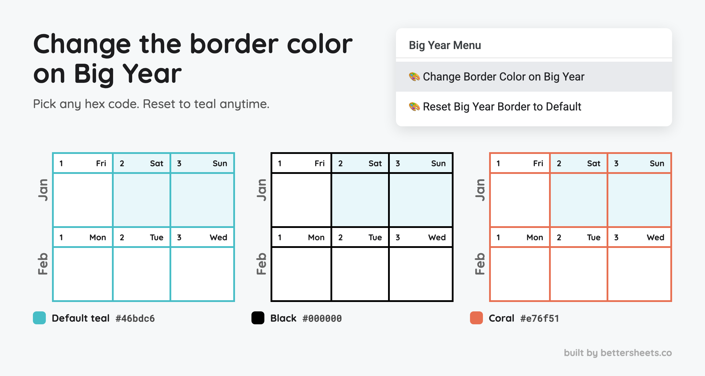
I just added a new feature to Big Year Premium: you can change the border color of the whole calendar. Click a menu button, type a hex code, and every border on the BIG tab turns that color. A second button puts the default teal back.

This post is the exact Apps Script behind it, written out step by step. You can copy it into your own sheet, or read along to learn how setBorder really works.

TL;DR

• Google Sheets has no “change only the border color” button, and neither does Apps Script. You have to redraw the borders in the new color.
• The trick is setBorder() with null: null means “leave this side alone”, so you can redraw exactly the sides you want and nothing else.
• Map where your borders are, put those ranges in a RangeList, and one call recolors hundreds of cells in a second.

What you’ll build

Two buttons in a custom menu:

1. Change Border Color on Big Year: asks for a hex code like #000000, then redraws every border on the tab in that color.
2. Reset Big Year Border to Default: puts the original teal (#46bdc6) back.

Everything here is Google Apps Script, the JavaScript-based language built into Google Sheets. You don’t need to install anything.

Why you can’t just “change the border color”

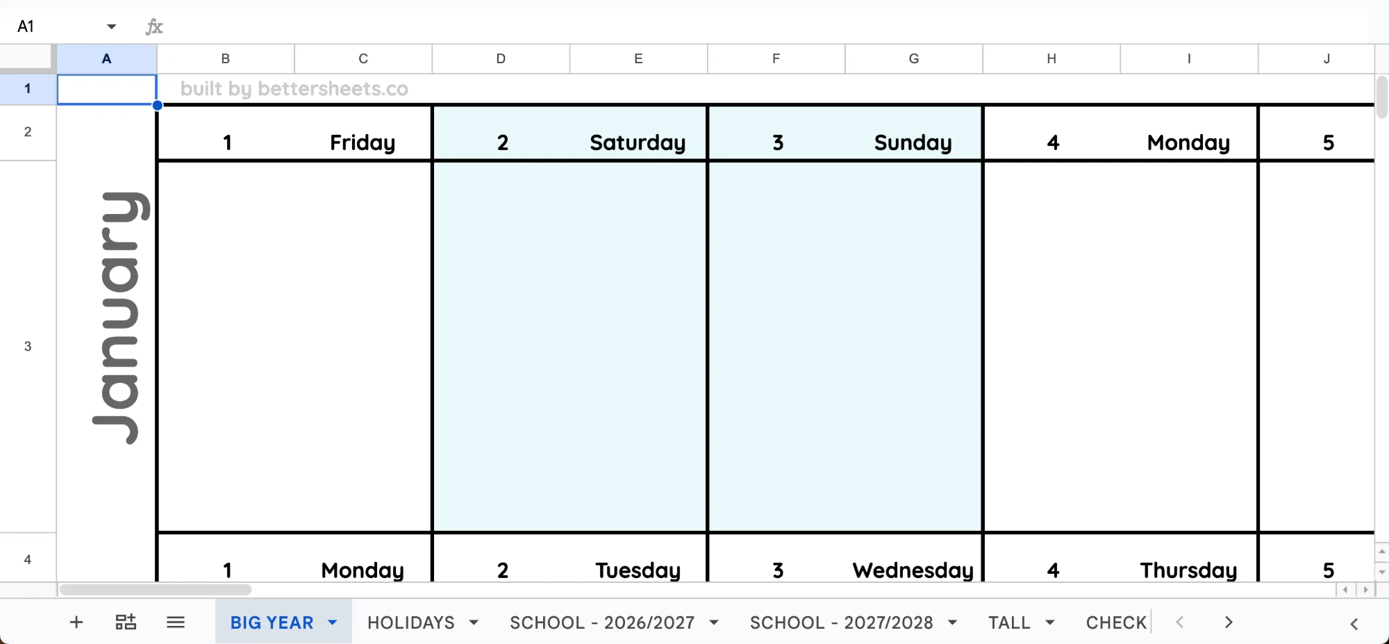
Here’s what Big Year looks like out of the box: thick teal borders around every day.

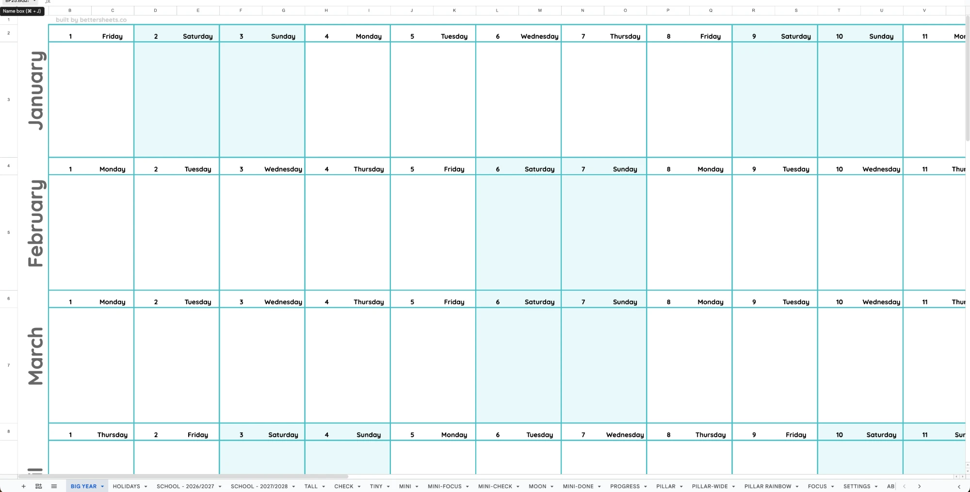
The obvious move is to select the whole calendar and pick a new border color. That doesn’t work. In Google Sheets, the border color you pick only applies to the next borders you draw. To recolor, you have to draw the borders again, and if you select everything and click “all borders”, you get borders on every single cell, including ones that never had them.

Apps Script has the same problem. range.setBorder() applies the same borders to the whole range you give it. There’s no “find every cell with a border and only change its color” function. (range.getBorder() can read borders, but only one cell at a time, so scanning a whole sheet that way is slow.)

So instead of searching for borders, we tell the script exactly where they are.

Step 1: Open the Apps Script editor

1. Open your Google Sheet.
2. In the menu, click Extensions → Apps Script.
3. A new tab opens with a file called Code.gs. This is where all the code in this post goes.
4. If Code.gs already has code in it (Big Year Premium does), scroll to the bottom and paste below it. Don’t delete what’s there.

Step 2: Map exactly where your borders are

This is the step that makes everything else easy. Look at your sheet and write down the pattern.

For Big Year, the borders start at B2 and end at BK25:

• Columns B to BK are 31 days. Each day is two columns wide: B:C is day 1, D:E is day 2, and so on up to BJ:BK for day 31.
• Rows 2 to 25 are 12 months. Each month is two rows: the date row (2, 4, 6…) and the box below it where you write (3, 5, 7…).

The box you write in is one merged cell with a border on all four sides. Easy.

The date row is the tricky part. It’s two cells: the day number on the left and the weekday on the right. Together they look like one box, but there’s no line between them. So each cell has only three of its four borders.

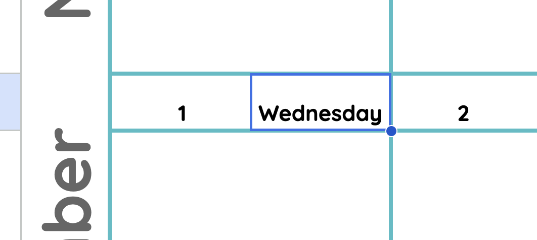
• The number cell (like B2) has a top, left and bottom border. No right border.
• The weekday cell (like C2) has a top, right and bottom border. No left border.

If we redrew those cells with all four sides, we’d add a line down the middle of every date. That’s why we need the next step.

Step 3: Understand setBorder’s eight arguments

setBorder takes eight arguments, in this order:

Apps Script · Code.gs

range.setBorder(top, left, bottom, right, vertical, horizontal, color, style);

• top, left, bottom, right: the outside edges of the range
• vertical: the inside lines between columns
• horizontal: the inside lines between rows
• color: a hex code like '#46bdc6'
• style: the line style, like SpreadsheetApp.BorderStyle.SOLID_THICK

Each of the first six can be one of three values:

• true: draw this border
• false: remove this border
• null: leave this border exactly as it is

That null is the whole trick. For the number cell we draw top, left and bottom, and pass null for right, so the middle of the date stays open:

Apps Script · Code.gs

numberCell.setBorder(true, true, true, null, null, null, '#000000', SpreadsheetApp.BorderStyle.SOLID_THICK);

Step 4: Find your current border color and style

You need two things before writing the real code: the hex code of your default color (so the reset button can put it back) and the line style (so the new borders are the same thickness).

Paste this into Code.gs. It reads the borders of four cells and prints what it finds:

Apps Script · Code.gs

function logBigYearBorderColor() {
  const sheet = SpreadsheetApp.getActive().getSheetByName('BIG YEAR');
  ['B2', 'C2', 'B3', 'C3'].forEach(a1 => {
    const b = sheet.getRange(a1).getBorder();
    if (!b) { Logger.log(a1 + ': no borders'); return; }
    ['Top', 'Left', 'Bottom', 'Right'].forEach(side => {
      const border = b['get' + side]();
      if (!border) return;
      Logger.log(a1 + ' ' + side + ': ' + border.getBorderStyle() + ' ' +
        border.getColor().asRgbColor().asHexString());
    });
  });
}

To run it:

1. Click the Save icon (or press Cmd+S / Ctrl+S).
2. In the toolbar, pick logBigYearBorderColor from the function dropdown.
3. Click Run.
4. The first time, Google asks for permission. Click Review permissions, pick your Google account, click Advanced, then Go to (your project name) (unsafe), then Allow. This is normal for your own scripts. “Unsafe” only means Google hasn’t reviewed it.
5. The results show up in the Execution log at the bottom.

Here’s what Big Year printed:

Execution log

B2 Top: SOLID_THICK #46bdc6
B2 Left: SOLID_THICK #46bdc6
B2 Bottom: SOLID_THICK #46bdc6
C2 Top: SOLID_THICK #46bdc6
C2 Bottom: SOLID_THICK #46bdc6
C2 Right: SOLID_THICK #46bdc6
B3 Left: SOLID_THICK #46bdc6
B3 Bottom: SOLID_THICK #46bdc6
B3 Right: SOLID_THICK #46bdc6
C3: no borders

Three things this told me:

• The default color is #46bdc6 and the style is SOLID_THICK.
• B2 and C2 really do have three sides each, just like the map in step 2.
• C3 has no borders because B3:C3 is one merged cell. The borders live on B3.

Gotcha: B3 has no top border, even though there’s clearly a line above it. That line is stored as B2’s bottom border. When two cells share an edge, Sheets can store it on just one of them. My first version of this function only asked for B3’s top border, got null, and crashed with TypeError: Cannot read properties of null (reading 'getColor'). Checking all four sides of a few cells avoids that.

Once you have your color and style, you can delete this function. It was only for looking.

Step 5: Set up the constants

Paste this at the top of your new code. These are the three values the rest of the script uses:

Apps Script · Code.gs

const BIG_YEAR_SHEET = 'BIG YEAR';
const BIG_YEAR_BORDER_STYLE = SpreadsheetApp.BorderStyle.SOLID_THICK;
const BIG_YEAR_DEFAULT_BORDER = '#46bdc6';

• BIG_YEAR_SHEET is the tab name, spelled exactly as it appears on the tab.
• BIG_YEAR_BORDER_STYLE matches what step 4 printed.
• BIG_YEAR_DEFAULT_BORDER is the default color. Hardcoding it means the reset button always knows where to go back to.

Step 6: Write the function that redraws the borders

This function does the actual work. Give it a hex code and it redraws every border on the tab in that color:

Apps Script · Code.gs

function applyBigYearBorderColor_(hex) {
  const sheet = SpreadsheetApp.getActive().getSheetByName(BIG_YEAR_SHEET);

  const numberCells = [];  // top, left, bottom
  const weekdayCells = []; // top, right, bottom
  const bodyCells = [];    // full box

  for (let month = 0; month < 12; month++) {
    const dateRow = 2 + month * 2;
    for (let day = 0; day < 31; day++) {
      const numCol = 2 + day * 2;
      numberCells.push(sheet.getRange(dateRow, numCol).getA1Notation());
      weekdayCells.push(sheet.getRange(dateRow, numCol + 1).getA1Notation());
      bodyCells.push(sheet.getRange(dateRow + 1, numCol, 1, 2).getA1Notation());
    }
  }

  sheet.getRangeList(numberCells).setBorder(true, true, true, null, null, null, hex, BIG_YEAR_BORDER_STYLE);
  sheet.getRangeList(weekdayCells).setBorder(true, null, true, true, null, null, hex, BIG_YEAR_BORDER_STYLE);
  sheet.getRangeList(bodyCells).setBorder(true, true, true, true, null, null, hex, BIG_YEAR_BORDER_STYLE);
}

Line by line:

1. Three empty lists, one for each border shape: number cells, weekday cells and the boxes underneath.
2. The outer loop goes through the 12 months. dateRow = 2 + month * 2 gives rows 2, 4, 6… up to 24.
3. The inner loop goes through the 31 days. numCol = 2 + day * 2 gives columns 2, 4, 6… (B, D, F…).
4. For each day, we add three addresses to the lists:
   • the number cell, like B2
   • the weekday cell one column to the right, like C2
   • the box underneath, two columns wide, like B3:C3
5. Three setBorder calls, one per shape. getRangeList() takes the whole list of addresses, so each call draws hundreds of cells at once. That’s why it finishes in about a second instead of a minute.

Look at the nulls:

• Number cells: true, true, true, null. Top, left and bottom are drawn. The right side is left alone.
• Weekday cells: true, null, true, true. Top, bottom and right are drawn. The left side is left alone.
• Boxes: true, true, true, true. All four sides.
• vertical and horizontal are null everywhere, so nothing inside a range changes.

The underscore at the end of applyBigYearBorderColor_ makes the function private. It won’t show up in the Run dropdown, and users can’t call it directly. Only the two functions below can.

Step 7: Ask for a hex code

This is the function the first menu button runs. It asks for a color, checks it, and passes it to the redraw function:

Apps Script · Code.gs

function changeBorderColorOnBigYearTab() {
  const ui = SpreadsheetApp.getUi();
  const res = ui.prompt('Border color', 'Enter a hex code, e.g. #46bdc6', ui.ButtonSet.OK_CANCEL);
  if (res.getSelectedButton() !== ui.Button.OK) return;

  let hex = res.getResponseText().trim();
  if (!hex.startsWith('#')) hex = '#' + hex;
  if (!/^#[0-9a-f]{6}$/i.test(hex)) {
    ui.alert('Not a valid hex code: ' + hex);
    return;
  }
  applyBigYearBorderColor_(hex);
}

What each part does:

1. ui.prompt(...) shows a small box with OK and Cancel buttons.
2. If you click Cancel (or close the box), the function stops. Nothing changes.
3. .trim() removes stray spaces, in case you pasted " #000000 ".
4. If you typed 000000 without the #, it adds the # for you.
5. The pattern /^#[0-9a-f]{6}$/i checks for exactly six hex characters. Upper or lower case both work. If it doesn’t match, you get an alert and nothing changes.
6. If it passes, the borders are redrawn.

Step 8: The reset button

The second menu button is one line, because the default color is already saved as a constant:

Apps Script · Code.gs

function defaultBorderOnBigYear() {
  applyBigYearBorderColor_(BIG_YEAR_DEFAULT_BORDER);
}

Step 9: Add the buttons to a custom menu

onOpen runs every time the sheet opens and builds the menu:

Apps Script · Code.gs

function onOpen() {
  SpreadsheetApp.getUi().createMenu('Big Year Menu')
    .addItem('🎨 Change Border Color on Big Year', 'changeBorderColorOnBigYearTab')
    .addItem('🎨 Reset Big Year Border to Default', 'defaultBorderOnBigYear')
    .addToUi();
}

Important: a project can only have one onOpen. If your sheet already has one (Big Year Premium does, with a bunch of other menu items), don’t paste a second one. Add just the two .addItem(...) lines inside the one you already have.

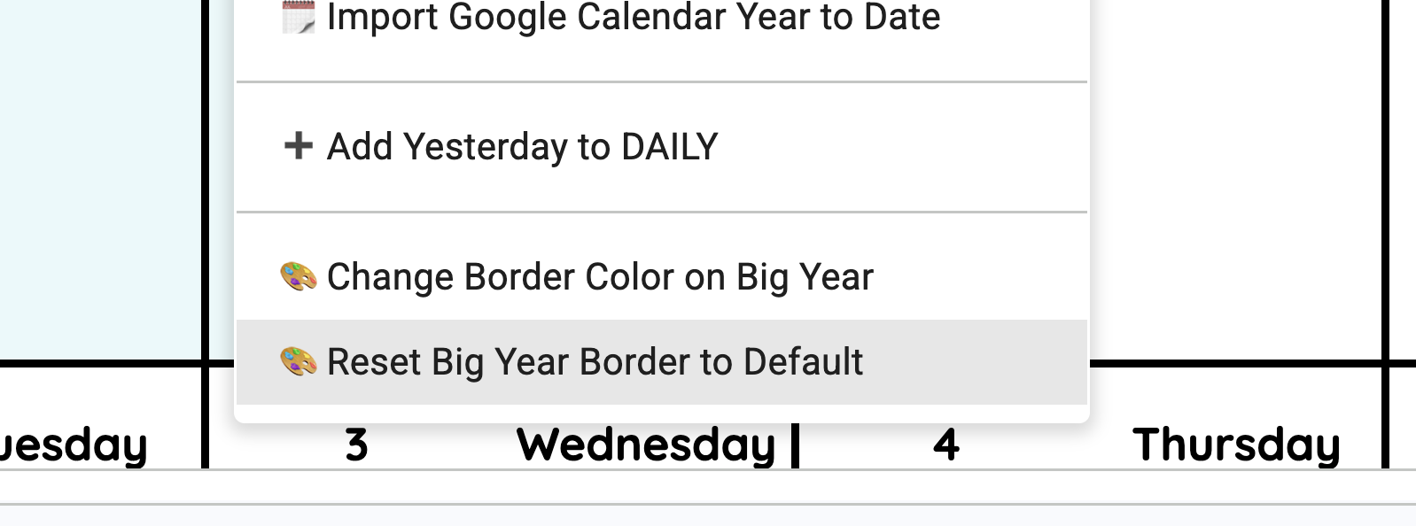
Save, then reload the Google Sheet. The menu shows up in the menu bar after a few seconds.

Step 10: Test it

1. Click Big Year Menu → 🎨 Change Border Color on Big Year.
2. Type a loud color like #000000 and click OK.
3. Check the date rows. The number and weekday should still share one box, with no line between them.
4. Scroll to the end of a short month, like February, and check the empty days too (more on that below).
5. Click 🎨 Reset Big Year Border to Default and make sure the teal comes back.

The bug I hit: empty days have borders too

My first version skipped any day block without a date in it. February has no 30th, so why draw a border there? The line looked like this:

Apps Script · Code.gs

if (values[dateRow - 2][numCol - 2] === '') continue; // no date = no box

That was wrong. The empty blocks at the end of short months still have borders. They just don’t have dates. After running the script, February 29 to 31 and every month’s missing 31st were still teal:

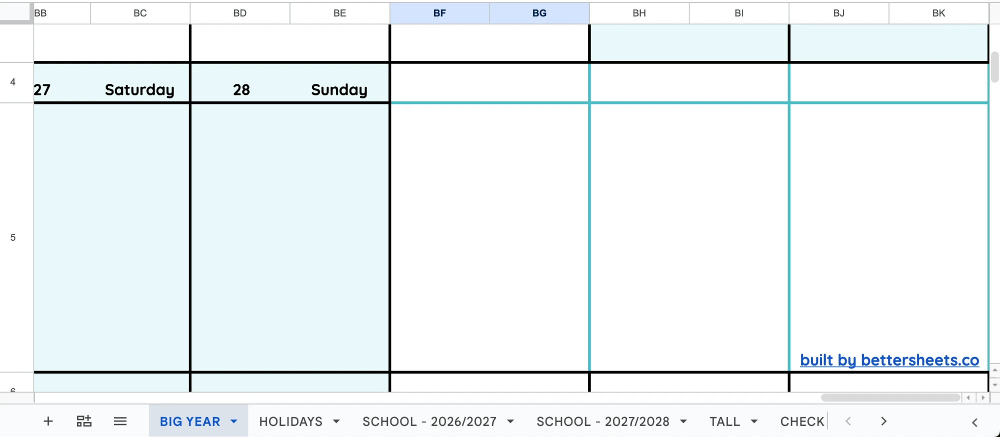
The fix was to delete that line and draw all 31 blocks for all 12 months, every time. The layout is the same in every month, so the code shouldn’t care what’s in the cells. That also means the script doesn’t need to read the sheet’s values at all.

Adapting this to your own sheet

The code above is written for Big Year’s layout, but the method works for any sheet with a repeating pattern:

1. Map your borders. Write down which cells have which sides. Look for repeats: every two columns, every three rows, and so on.
2. Group cells by shape. Each group gets its own list and its own setBorder call, with null for the sides you don’t want touched.
3. Read your style and color first with the logging function from step 4, so the new borders match.
4. Test on a copy of your sheet before you run it on the real one.
5. Check the edges: the last row, the last column, and any empty blocks.

Color ideas

Once it works, here are some hex codes to try:

• #000000 black, bold and clean
• #FFFFFF white, which makes the lines vanish
• #9B111E ruby red
• Team colors: Man United #DA020E, Arsenal #EF0107, Philadelphia Eagles #004C54, Chelsea #034694
• School colors: Michigan #00274C, Harvard #A51C30
• Your brand color, so your planner matches your logo

The full script

Here’s everything in one block, ready to paste into Code.gs. If you already have an onOpen, leave that function out and add the two menu lines to yours.

Apps Script · Code.gs

const BIG_YEAR_SHEET = 'BIG YEAR';
const BIG_YEAR_BORDER_STYLE = SpreadsheetApp.BorderStyle.SOLID_THICK;
const BIG_YEAR_DEFAULT_BORDER = '#46bdc6';

function onOpen() {
  SpreadsheetApp.getUi().createMenu('Big Year Menu')
    .addItem('🎨 Change Border Color on Big Year', 'changeBorderColorOnBigYearTab')
    .addItem('🎨 Reset Big Year Border to Default', 'defaultBorderOnBigYear')
    .addToUi();
}

function changeBorderColorOnBigYearTab() {
  const ui = SpreadsheetApp.getUi();
  const res = ui.prompt('Border color', 'Enter a hex code, e.g. #46bdc6', ui.ButtonSet.OK_CANCEL);
  if (res.getSelectedButton() !== ui.Button.OK) return;

  let hex = res.getResponseText().trim();
  if (!hex.startsWith('#')) hex = '#' + hex;
  if (!/^#[0-9a-f]{6}$/i.test(hex)) {
    ui.alert('Not a valid hex code: ' + hex);
    return;
  }
  applyBigYearBorderColor_(hex);
}

function defaultBorderOnBigYear() {
  applyBigYearBorderColor_(BIG_YEAR_DEFAULT_BORDER);
}

function applyBigYearBorderColor_(hex) {
  const sheet = SpreadsheetApp.getActive().getSheetByName(BIG_YEAR_SHEET);

  const numberCells = [];  // top, left, bottom
  const weekdayCells = []; // top, right, bottom
  const bodyCells = [];    // full box

  for (let month = 0; month < 12; month++) {
    const dateRow = 2 + month * 2;
    for (let day = 0; day < 31; day++) {
      const numCol = 2 + day * 2;
      numberCells.push(sheet.getRange(dateRow, numCol).getA1Notation());
      weekdayCells.push(sheet.getRange(dateRow, numCol + 1).getA1Notation());
      bodyCells.push(sheet.getRange(dateRow + 1, numCol, 1, 2).getA1Notation());
    }
  }

  sheet.getRangeList(numberCells).setBorder(true, true, true, null, null, null, hex, BIG_YEAR_BORDER_STYLE);
  sheet.getRangeList(weekdayCells).setBorder(true, null, true, true, null, null, hex, BIG_YEAR_BORDER_STYLE);
  sheet.getRangeList(bodyCells).setBorder(true, true, true, true, null, null, hex, BIG_YEAR_BORDER_STYLE);
}

Skip the code: get it in Big Year Premium

If you want a yearly calendar with this already built in, it’s in Big Year Premium. It’s $10, or free for Lifetime members. You get the BIG tab with the border color buttons, plus a dozen more yearly layouts and sync from Google Calendar.

Just want the calendar? Big Year is free: the whole year on one tab, printable and editable.